[Formats: html | pdf | kindle pdf]
Locality-sensitive hashing (LSH) is a set of techniques that dramatically speed up search-for-neighbors or near-duplication detection on data. These techniques can be used, for example, to filter out duplicates of scraped web pages at an impressive speed, or to perform near-constant-time lookups of nearby points from a geospatial data set.
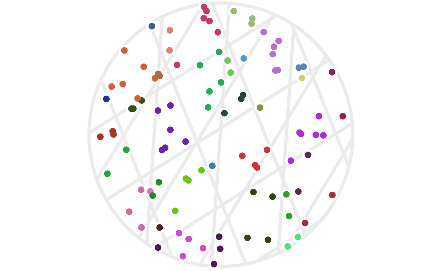
Figure 1: A preview of LSH in action. Only hash collisions were used to find the weights in this image — no pairwise distances were explicitly computed.
Let’s take a quick look at other types of hash functions to get a bird’s-eye view of what counts as a hash function, and how LSH fits into that world. A traditional use for hash functions is in hash tables. As a reminder, the hash functions used in a hash table are designed to map a piece of data to an integer that can be used to look in a particular bucket within the hash table to retrieve or delete that element. Many containers with string keys, such as JavaScript objects or Python dictionaries, are based on hash tables. Although hash tables might not guarantee constant-time lookups, in practice they effectively provide them.
There are other classes of hash functions as well. For example, the SHA-1 cryptographic hash function is designed to be difficult to reverse, which is useful if you want to store someone’s password as a hashed value. Hash functions like these are called cryptographic hash functions.
Hash functions typically have these key properties:
- They map some type of input, such as strings or floats, to discrete values, such as integers.
- They’re designed so that two inputs will result in hash outputs that are either different or the same based on key properties of the inputs.
Here’s how LSH fits in: Locality-sensitive hash functions are specifically designed so that hash value collisions are more likely for two input values that are close together than for inputs that are far apart. Just as there are different implementations of secure hash functions for different use cases, there are different implementations of LSH functions for different data types and for different definitions of being close together. I’ll use the terms neighbors or being nearby to refer to points that we deem “close enough” together that we’d want to notice their similarity. In this post, I’ll give a brief overview of the key ideas behind LSH and take a look at a simple example based on an idea called random projections, which I’ll define in section 2 below.
1 A human example
It will probably be much easier to grasp the main idea behind LSH with an example you can relate to. This way we can build some intuition before diving into those random projections that we’ll use in the next section.
Suppose you have a million people from across the United States all standing in a huge room. It’s your job to get people who live close together to stand in their own groups. Imagine how much time it would take to walk up to each person, ask for their street address, map that to a lat/long pair, then write code to find geographic clusters, and walk up to every person again and tell them how to find the rest of their cluster. I cringe just thinking about the time complexity.
Here’s a much better way to solve this problem: Write every U.S. zip code on poster boards and hang those from the ceiling. Then tell everyone to go stand under the zip code where they live.
Voila! That’s much easier, right? That’s also the main idea behind LSH. We’re taking an arbitrary data type (a person, who we can think of as a ton of data including their street address), and mapping that data into a set of discrete values (zip codes) such that people who live close together probably hash to the same value. In other words, the clusters (people with the same zip code) are very likely to be groups of neighbors.
A nice benefit of the zip code approach is that it’s parallel-friendly. Instead of requiring a center of communication, every person can walk directly to their destination without further coordination. This is a bit surprising in light of the fact that the result (clusters of neighbors) is based entirely on the relationships between the inputs.
Another property of this example is that it is approximate: some people may live across the street from each other, but happen to have different zip codes, in which case they would not be clustered together here. As we’ll see below, it’s also possible for data points to be clustered together even when they’re very far apart, although a well-designed LSH can at least give some mathematical evidence that this will be a rare event, and some implementations manage to guarantee this can never happen.
2 Hashing points with projections
In this section, I’ll explain exactly how a relatively straightforward LSH approach works, explore some key parameters for this LSH system, and review why this technique is an order of magnitude faster than some other approaches.
Let’s start with an incredibly simple mathematical function that we can treat as an LSH. Define \(h_1:{\mathbb{R}}^2 \to {\mathbb{Z}}\) for a point \(x=(x_1, x_2)\in{\mathbb{R}}^2\) by
\[ h_1(x) := \lfloor x_1 \rfloor; \]
that is, \(h_1(x)\) is the largest integer \(a\) for which \(a\le x_1.\) For example, \(h_1((3.2, -1.2)) = 3.\)
Let’s suppose we choose points at random by uniformly sampling from the origin-centered circle \(\mathcal C\) with radius 4:
\[ \mathcal C := \{ (x, y) : x^2 + y^2 \le 4^2 \}. \]
Suppose we want to find which of our points in \(\mathcal C\) are close together. We can estimate this relationship by considering points \(a, b \in \mathcal C\) to be clustered together when \(h_1(a) = h_1(b).\) It will be handy to introduce the notation \(a \sim b\) to indicate that \(a\) and \(b\) are in the same cluster. With that notation, we can write our current hash setup as
\[ a \sim b \iff h_1(a) = h_1(b). \]
Figure 2 shows an example of such a clustering.
Figure 2: Twenty points chosen randomly in a circle with radius 4. Each point \(x\) is colored based on its hash value \(h_1(x).\)
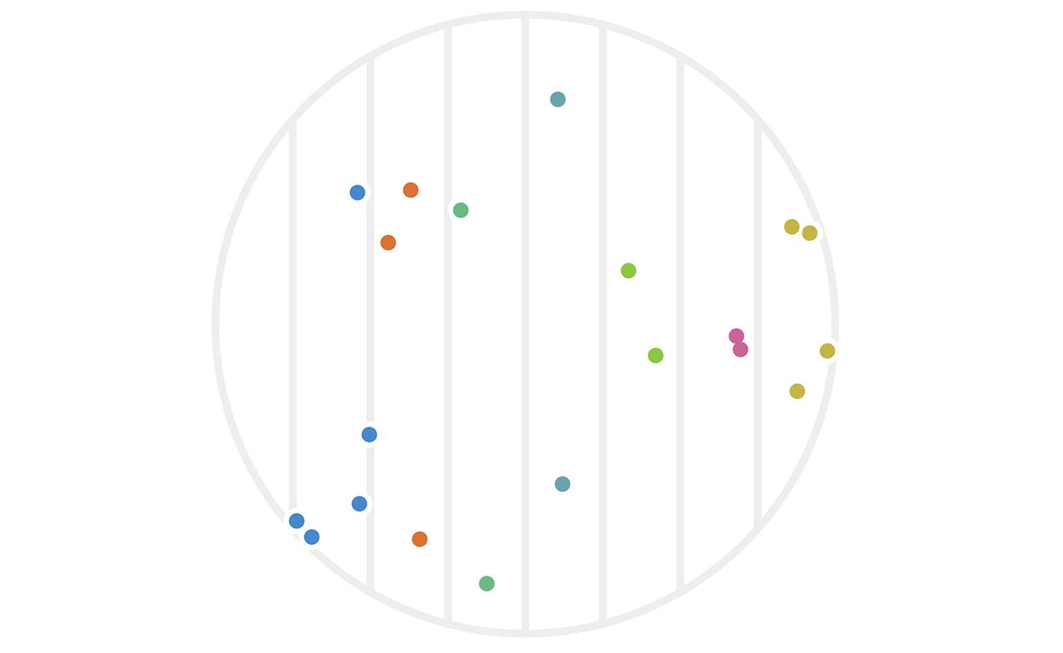
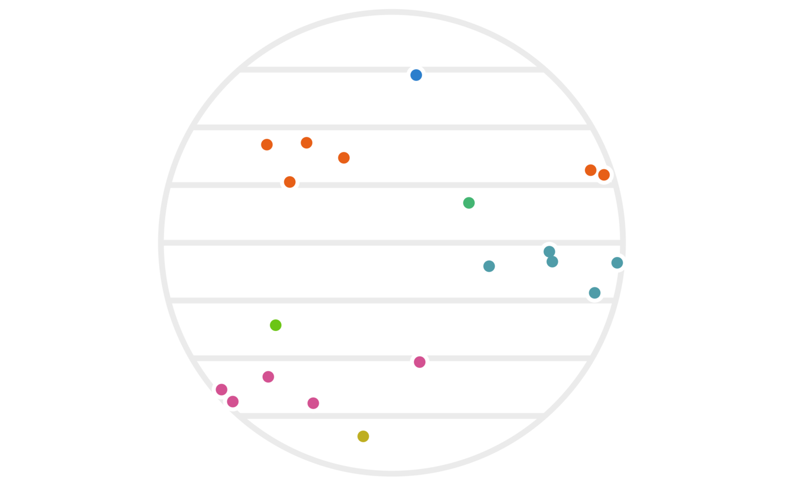
You can immediately see that some points are far apart yet clustered, while others are relatively close yet unclustered. There’s also a sense that this particular hash function \(h_1\) was arbitrarily chosen to focus on the x-axis. What would have happened with the same data if we had used instead \(h_2(x) := \lfloor x_2 \rfloor?\) The result is figure 3.
Figure 3: The same twenty points as figure 1, except that we’re using the \(y\) values (instead of \(x\) values) to determine the hash-based cluster colors this time around.
While neither clustering alone is amazing, things start to work better if we use both of them simultaneously. That is, we can redefine our clustering via
\[ a \sim b \iff \begin{cases} h_1(a) = h_1(b), \text{and} \\ h_2(a) = h_2(b). \\ \end{cases} {\class{smallscrneg}{ }}\qquad(1)\]
Our same example points are shown under this new clustering in figure 4.
Figure 4: The same twenty points clustered via two different hashes — one using \(\lfloor x\rfloor\), the other using \(\lfloor y\rfloor.\) As before, points are colored based on which cluster they’re in; a cluster is the set of all points who share both their \(\lfloor x\rfloor\) and their \(\lfloor y\rfloor\) values.
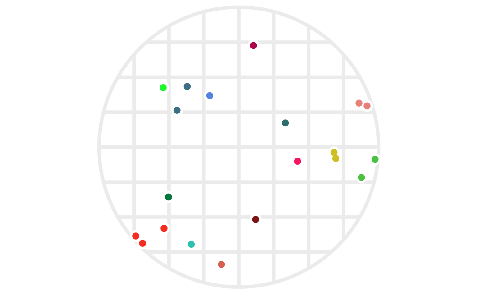
This does a much better job of avoiding clusters with points far apart, although, as we’ll see below, we can still make some improvements.
2.1 Randomizing our hashes
So far we’ve defined deterministic hash functions. Let’s change that by choosing a random rotation matrix \(U\) (a rotation around the origin) along with a random offset \(b \in [0, 1).\) Given such a random \(U\) and \(b,\) we could define a new hash function via
\[ h(x) := \lfloor (Ux)_1 + b \rfloor, \]
where I’m using the notation \(( \textit{vec} )_1\) to indicate the first coordinate of the vector value vec. (That is, the notation \((Ux)_1\) means the first coordinate of the vector \(Ux\).) This function is the random projection I referred to earlier.
It may seem a tad arbitrary to use only the first coordinate here rather than any other, but the fact that we’re taking a random rotation first means that we have the same set of possibilities, with the same probability distribution, as we would when pulling out any other single coordinate value.
A key advantage of using randomized hash functions is that any probabilistic statements we want to make about performance (e.g., “99% of the time this algorithms will give us the correct answer”) applies equally to all data, as opposed to applying to some data sets but not to others. As a counterpoint, consider the way quicksort is typically fast, but ironically uses \(O(n^2)\) time to sort a pre-sorted list; this is a case where performance depends on the data, and we’d like to avoid that. If we were using deterministic hash functions, then someone could choose the worst-case data for our hash function, and we’d be stuck with that poor performance (for example, choosing maximally-far apart points that are still clustered together by our \(h_1\) function above). By using randomly chosen hash functions, we can ensure that any average-case behavior of our hash functions applies equally well to all data. This same perspective is useful for hash tables in the form of universal hashing.
Let’s revisit the example points we used above, but now apply some randomized hash functions. In figure 4, points are clustered if and only if both of their hash values (from \(h_1(x)\) and \(h_2(x)\)) collide. We’ll use that same idea, but this time choose four rotations \(U_1, \ldots, U_4\) as well as four offsets \(b_1, \ldots, b_4\) to define \(h_1(), \ldots, h_4()\) via
\[ h_i(x) := \lfloor (U_i x)_1 + b_i \rfloor. \qquad(2)\]
Figure 5 shows the resulting clustering. This time, there are 100 points since using more hash functions has effectively made the cluster areas smaller. We need higher point density to see points that are clustered together now.
Figure 5: One hundred random points clustered using four random hash functions as defined by (2). Points have the same color when all four of their hash values are the same. Each set of parallel light gray lines delineates the regions with the same hash value for each of the \(h_i()\) functions.
It’s not obvious that we actually want to use all four of our hash functions. The issue is that our clusters have become quite small. There are a couple ways to address this. One is to simply increase the scale of the hash functions; for example, set:
\[ \tilde h_i(x) := h_i(x/s), \]
where \(s\) is a scale factor. In this setup, larger \(s\) values will result in larger clusters.
However, there is something a bit more nuanced we can look at, which is to allow some adaptability in terms of how many hash collisions we require. In other words, suppose we have \(k\) total hash functions (just above, we had \(k=4\)). Instead of insisting that all \(k\) hash values must match before we say two points are in the same cluster, we could look at cases where some number \(j \le k\) of them matches. To state this mathematically, we would rewrite equation (1) as
\[ a \sim b \iff \#\{i: h_i(a) = h_i(b)\} \ge j. {\class{smallscrneg}{ }}\qquad(3)\]
Something interesting happens here, which is that the \(a \sim b\) relationship is no longer a clustering, but becomes more like adjacency (that is, sharing an edge) in a graph. The difference is that, in a clustering, if \(a\sim b\) and \(b\sim c,\) then we must have \(a\sim c\) as well; this is called being transitively closed. Graphs don’t need to have this property. Similarly, it’s no longer true that our similarity relationship \(a\sim b\) is transitively closed.
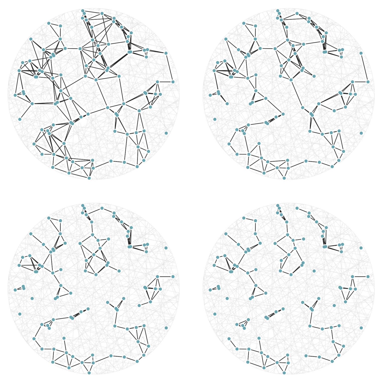
It may help your intuition to see this new definition of \(a\sim b\) in action on the same 100 points from figure 5. This time, in figure 6, there are twenty random hashes, and we’re seeing the graphs generated by equation (3) using cutoff values (values of \(j\)) of 6, 7, 8, and 9. The top-left graph in figure 6 has an edge drawn between two points \(a\) and \(b\) whenever there are at least 6 hash functions \(h_i()\) with \(h_i(a) = h_i(b),\) out of a possible 20 used hash functions.
Figure 6: A set of 100 random points with graph edges drawn according to (3). There are 20 random hash functions used. The top-left graph uses the cutoff value \(j=6.\) The remaining three graphs, from top-left to bottom-right, have cutoff values \(j=7,\) 8, and 9 respectively; this means each graph is a subgraph (having a subset of the edges) of the previous one.
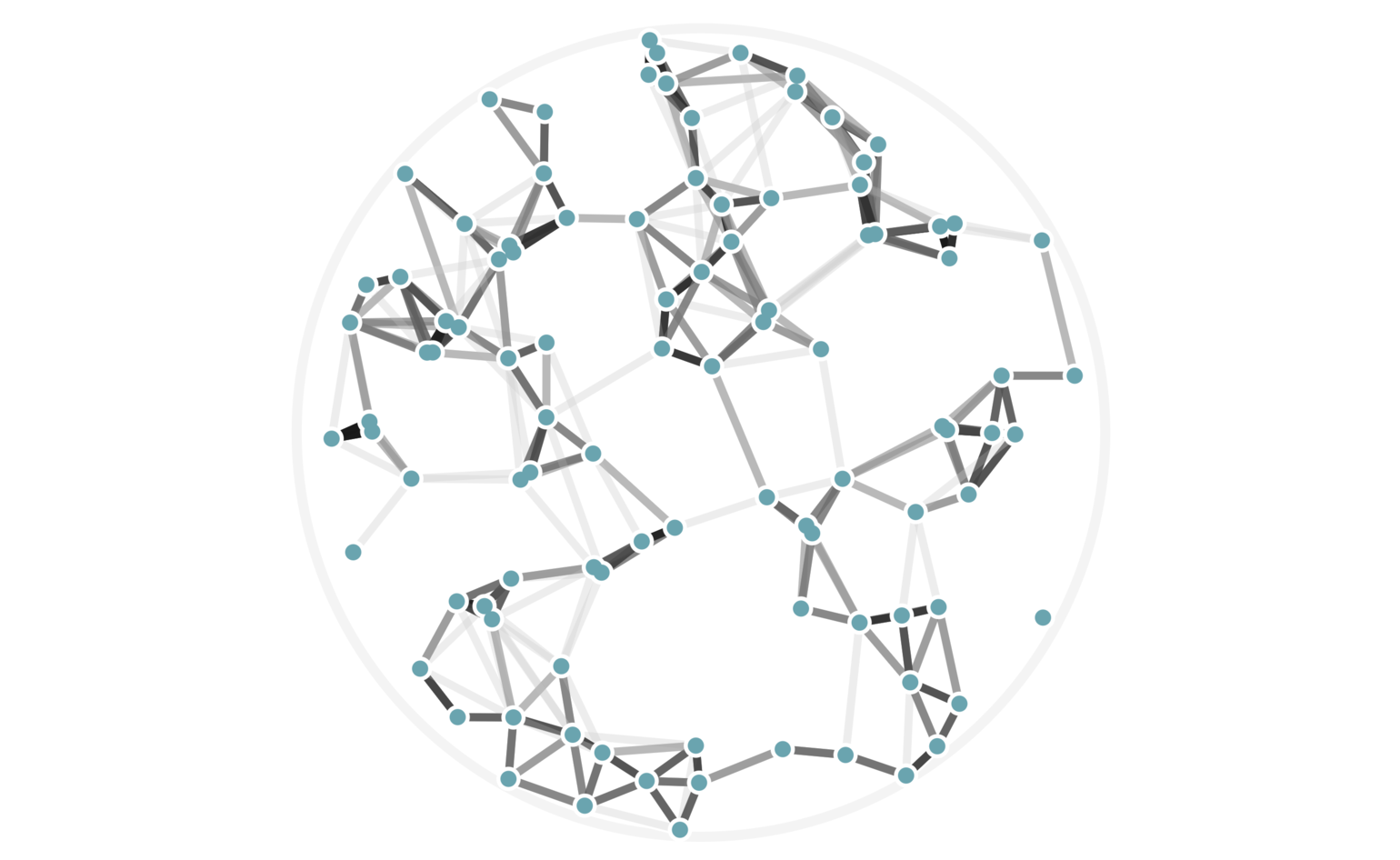
In fact, we can visualize all possible cutoff values of 6 or higher — these are values of \(j\) in equation (3) — using a single image with weighted edges, as seen in figure 7. Keep in mind that we haven’t explicitly computed any pairwise distances to arrive at this data.
Figure 7: The same 100 random points from figure 6, this time rendered with edge weights that depend on how many hash collisions are present between any two points. A black edge represents the maximum of 20 hash collisions; the lightest edge represents only 6 hash collisions.
There’s another fun way to build intuition for what information our hashes provide. Let’s visualize regions of the circle where all points have the same number of hash collisions with a given query point. We can do this by showing an example query point \(q\), and shading each region based on the number of hash collisions the region’s points have with \(q\); this is shown in figure 8. Every point in each shaded region has the same hash values for all the hash functions used. The first part of figure 8 shows a scaled version of the two-hash system (using \(h_1()\) and \(h_2()\), similar to figure 4) that we saw before; the second part uses 5 random hashes. The darkest region contains points \(p\) where all hash values collide, so \(h_i(p) = h_i(q)\) for all \(i\). In a lightly shaded region that equation will only hold true for a smaller subset of the hash functions \(h_i().\)
The second part of figure 8 (with 5 hashes) shows nicer behavior, and I’ll try to explain why. Imagine that we were drawing these same images for some theoretically perfect LSH setup that somehow managed to match point \(q\) to every point \(p\) with \(||p-q||\le r\) for some radius \(r\); all other points were not matched. For that perfect LSH setup, images like figure 8 would show a fixed-size circle with center at \(q\) that moved along with \(q\). With that in mind as the perfect LSH result, notice that the second part in figure 8 is much closer to this ideal than the first part. Keep in mind that lookups within the shaded regions are no longer linear searches through data, but rather the intersection of \(k\) hash table lookups — that is, lookups of nearby points are significantly faster.
Figure 8: The first part shows the regions where points would be matched by either two (dark regions) or just one (lighter shade) hash collision with the moving query point \(q\). The second part shows the analogous idea for 5 random hash functions; in the latter case, the lightest shaded region indicates 3 hash collisions.
It may further help your intuition to see how weighted edges connecting a point to its neighbors, like those in figure 7, change as a single query point moives. This is the idea behind figure 9, where weighted edges are drawn between a moving query point and 100 random points. Notice that the edge weightings make intuitive sense: they tend to connect strongly to very close neighbors, weakly to farther neighbors, and not at all to points beyond a certain distance.
Figure 9: Edges weighted by how many hash collisions are present between the moving query point and 100 random points. Darker edges indicate more hash collisions. This image uses 12 random hashes, and requires at least 6 hash collisions for an edge to appear.
2.2 Choosing values of \(j\)
So far, we’ve seen that we can use hash lookups to find nearby neighbors of a query point, and that using \(k\) different randomized hash functions gives us much more accurate lookups than if we used a single hash function. An interesting property of figure 7 and figure 9 is that we used different numbers of hash collisions — via the variable \(j\) — to discover different degrees of similarity between points. In many applications, such as finding near duplicates or close geospatial points, we only want a binary output, so we have to choose a particular value for \(j\). Let’s discuss how to choose good values for \(j.\)
Suppose \(k\) is fixed. How can we decide which value of \(j\) is best?
To answer this question, let’s temporarily consider what a perfect function would do for us. We’ll call this function search(q). In an ideal world this function returns all points within a fixed distance of the query point. We could visualize this as an \(n-\)dimensional sphere around the query point \(q\). A call to search(q) ought to return all the indexed points \(p\) that live within this sphere.
Let’s move from that idealized algorithm into our fast-but-approximate world of locality-sensitive hashes. With this approach, there is no exact cutoff distance, although we keep the property that nearby neighbors are very likely to be in the returned list and distant points are very likely to be excluded. Since our hash functions are randomized, we can think of the neighbor relationship \(p\sim q\) as being a random variable that has a certain probability of being true or false once all our parameters are fixed (as a reminder, our main parameters are \(j\) and \(k\)).
Now consider what great performance looks like in the context of this random variable. Ideally, there is some distance \(D\) such that
\[||p-q|| < D-\varepsilon {\quad{\class{smallscr}{\hskip -0.8em}}}\Rightarrow{\quad{\class{smallscr}{\hskip -0.8em}}}P(p\sim q) > 1 - \delta;\] \[||p-q|| > D+\varepsilon {\quad{\class{smallscr}{\hskip -0.8em}}}\Rightarrow{\quad{\class{smallscr}{\hskip -0.8em}}}P(p\sim q) < \delta.\]
In other words, this distance \(D\) acts like a cutoff for our approximate search function. Points closer than distance \(D\) to query point \(q\) are returned, while points farther are not.
I wrote a Python script to calculate some of these probabilities for the particular parameters \(k=2\) and \(d=2\) (\(d\) is the dimensionality of the points), and for various values of \(j\). In particular, I restricted my input points to certain distances and measured the probability that they had at least \(j\) hash collisions for different \(j\) values. If you’re familiar with conditional probabilities, then this value can be written as:
\[ P\big(p \sim_j q \, \big| \, ||p-q|| = D\big), \]
where I’ve written \(p\sim_j q\) to denote that points \(p\) and \(q\) have at least \(j\) hash collisions.
Using this Python script, I’ve visualized the collision behavior of \(p\sim_j q\) for various \(j\) in figure 10. I’ll go into more detail about what each tick on the box plot indicates, but the intuition is that shorter box plots are better because in this visualization a shorter box plot indicates a smaller range of uncertainty.
Figure 10: Intuitively, each box plot represents the distances at which points \(p, q\) will achieve mixed results (sometimes classified as nearby, other times as not) from our LSH setup. A very short box plot is ideal because it indicates a smaller range of uncertainty. In other words, a short box plot corresponds to a setting in which most pairs of points are correctly classified by an LSH system as nearby or far apart based on their actual distance.
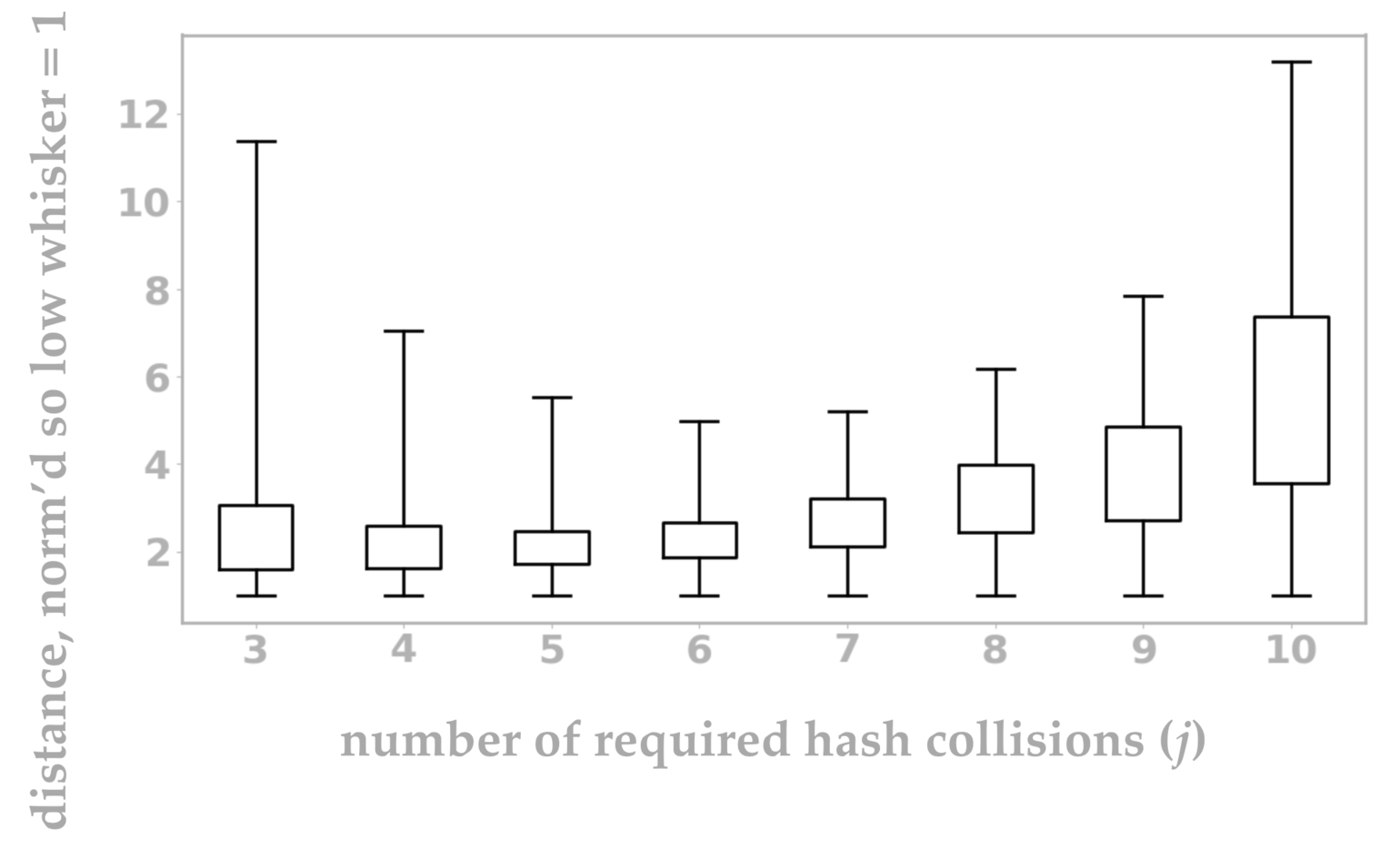
The most interesting element of this graph is that the best value of \(j\) appears to be \(j=6.\) You might have guessed that your best LSH approach is to insist that all of your random hashes must collide before you consider two points to be neighbors, but this measurement shows that intuition to be false.
So what exactly did we measure in figure 10? A traditional box plot visualizes the 25th and 75th percentiles of a set of scalar data points as the boundaries of the box. Often the median (50th percentile) is also shown within the box, but we don’t include an analogous mark in figure 10. The “whiskers” at either end may indicate the minimum and maximum values, or something similar such as the extreme values after removing outliers.
In our case, we have one box plot for each value of \(j\), and each plot has been normalized so that the bottom whiskers all align at value 1. (I’ll explain why this is useful in a moment.) The bottom whisker indicates the distance between \(p\) and \(q\) so that \(p\sim_j q\) is true 99% of the time. The bottom of the box is the relative distance at which \(p\sim_j q\) is true 75% of the time. Continuing in this pattern, the box top corresponds to the distance at which we get collisions 25% of the time, and the top whisker is the distance at which we get collisions 1% of the time. Since the box plots are all normalized (meaning that the distances per \(j\) value have all been divided through by the smallest distance), it’s easy to visually see the ratio of each box plot position versus its smallest distance. In other words, it’s easy to see which distance range is smallest.
Because I love math and precision, I’m going to provide one last definition to formalize the idea of figure 10. Given a value \(s \in (0, 1)\), define the distance \(D_s\) as the value satisfying the given equation:
\[ P\big(p \sim_j q \, \big| \, ||p-q|| = D_s\big) = s, \]
where \(p\sim_j q\) means that \(\#\{i : h_i(p) = h_i(q)\} \ge j.\) Intuitively, if \(\varepsilon\) is close to zero, then the distance \(D_\varepsilon\) is large because the probability of \(p\sim_j q\) is small. The value of \(D_{1/2}\) is the perfect distance so that \(p \sim_j q\) happens half of the time, and \(D_{1-\varepsilon}\) is a small distance where \(p \sim_j q\) happens almost all the time. Using this definition, the four values shown in each box plot of figure 10, from bottom to top, are:
\[D_{.99} / D_{.99} ,{\;\;{\class{smallscr}{\hskip -0.3em}}}D_{.75} / D_{.99} ,{\;\;{\class{smallscr}{\hskip -0.3em}}}D_{.25} / D_{.99} ,{\;\;{\class{smallscr}{\hskip -0.3em}}}D_{.01} / D_{.99}.\]
2.3 Why an LSH is faster
So far we’ve been sticking to 2-dimensional data because that’s easier to visualize in an article. However, if you think about computing 10 hashes for every 2-dimensional point in order to find neighbors, it may feel like you’re doing more work than the simple solution of a linear search through your points. Let’s review cases where using an LSH is more efficient than other methods of finding nearby points.
There are two ways an LSH can speed things up: by helping you deal with a huge number of points, or by helping you deal with points in a high-dimensional space such as image or video data.
2.3.1 An LSH is fast over many points
If you want to find all points close to a query point \(q,\) you could execute a full linear search. A single-hash LSH can give you results in constant time. That’s faster.
Things are slightly more complex for higher values of \(j\) and \(k.\) If you keep \(j=k,\) then your LSH result is a simple intersection of \(k\) different lists, each list being the set of hash collision points returned by a given randomized hash function \(h_i().\) Finding this intersection can be sped up by starting with the smallest of these lists and shrinking it by throwing out points not present in the other lists. This throwing-out process can be done quickly by using hash-table lookups to test for inclusion in the point lists, which are basically constant time. The running time of this approach is essentially \(O(mk),\) where \(m\) is the length of the shortest list returned by any of your hash functions \(h_i().\) This running time is very likely to be an order of magnitude faster than linear search.
2.3.2 An LSH is faster for high-dimensional points
There is a beautiful mathematical result called the Johnson-Lindenstrauss lemma which shows that random projections (which is what we’re using in our \(h_i()\) functions) are amazingly good at preserving point-wise distances (Dasgupta and Gupta 2003). As a result of this, you can often use a much smaller number of hash functions than your dimensionality \(d\) to set up an effective LSH system.
In particular, if you have \(n\) points, then you can use on the order of \(\log(n)\) hash functions and still achieve good results. With the \(j=k\) approach from the last section, a lookup would require \(O(m\log(n))\) time, where \(m\) is the length of the smallest list returned by your hash functions. Even if you wanted to take the more complex approach of setting \(j < k,\) you would still gain a speedup even on pairwise comparisons. Normally it requires \(O(d)\) time to compute the distance between two points. Using \(k \approx \log(n)\) hashes, it would instead take \(O(\log(n))\) time to compute the number of hash collisions between two points.
To show how significant this last speedup can be, imagine looking for copyright violations among movie files that are 1GB each. There have been about 500,000 movies made in the United States so far. With these numbers, we would require looking at 2 billion numeric values of data to directly compare two video files, versus looking at about 210 numeric values of data to compare their LSH values. (The value 210 is twice the expression \(8\log(500,000),\) which is a simplified suggested value for \(k\) from the Johnson-Lindenstrauss lemma.) The LSH approach here is about 10 million times faster.
3 Other data types and approaches
This article has focused on numeric, 2-dimensional data because it’s easier to visualize. Locality-sensitive hashes can certainly be used for many data types including strings, sets, or high-dimensional vectors.
Yet another ingredient to throw into the mix here is a set of techniques to boost performance tht treat an LSH as a black box. My favorite approach here is to simply perform multiple lookups on a hash system, each time using \(q + \varepsilon\) as an input, where \(q\) is your query value, and \(\varepsilon\) is a random variable centered at zero (Panigrahy 2006).
There’s a lot more that can be said about LSH techniques. If there is reader interest, I may write a follow-up article explaining the details of min-wise hashing, which is a fun case that’s simultaneously good at quickly finding nearby sets as well as nearby strings (Broder et al. 2000).
Hi! I hope you enjoyed my article. As you can see, I love building systems that get the most out of data. If you’d like to work together on a machine learning project, I’d love to hear from you. My company, Unbox Research, has a small team of talented ML engineers. We specialize in helping content platforms make more intelligent use of their data, which translates to algorithmic text and image comprehension as well as driving user engagement through discovery or personalization. Email me at tyler@unboxresearch.com.
References
Broder, Andrei Z, Moses Charikar, Alan M Frieze, and Michael Mitzenmacher. 2000. “Min-Wise Independent Permutations.” Journal of Computer and System Sciences 60 (3). Elsevier: 630–59.
Dasgupta, Sanjoy, and Anupam Gupta. 2003. “An Elementary Proof of a Theorem of Johnson and Lindenstrauss.” Random Structures & Algorithms 22 (1). Wiley Online Library: 60–65.
Panigrahy, Rina. 2006. “Entropy Based Nearest Neighbor Search in High Dimensions.” In Proceedings of the Seventeenth Annual Acm-Siam Symposium on Discrete Algorithm, 1186–95. Society for Industrial; Applied Mathematics.